What is ESMValCore API and using it in a Jupyter notebook
Overview
Teaching: 20 min
Exercises: 40 min
Compatibility: ESMValTool, ESMValCore v2.14.0Questions
How to find data for ESMValTool in a Jupyter Notebook?
How to use preprocessor functions?
Objectives
Use the Dataset object
Import and use preprocessor functions
View and check the data
In this episode we will introduce the ESMValCore API in a jupyter notebook. ESMValTool acts as a
wrapper and collection of recipes and diagnostics and CMORisers for observations that is built on
top of ESMValCore which has the core functionality.
A schematic overview is depicted below.
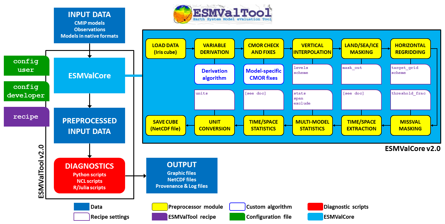 Using the functionalities in the ESMValCore light blue box in this modular way allows users to
use existing code to explore and build insights in the data and can help them build and write a
recipe and diagnostic script with the previous episodes Writing your own recipe / diagnostic script
Using the functionalities in the ESMValCore light blue box in this modular way allows users to
use existing code to explore and build insights in the data and can help them build and write a
recipe and diagnostic script with the previous episodes Writing your own recipe / diagnostic script
This episode is reformatted from material from this blog post by Peter Kalverla. There’s also material from the example notebooks and the API reference documentation.
Start JupyterLab
A jupyter notebook is an interactive document where you can run code alongside markdown cells for explanation text and images. All python code in this episode was written to be in a python cell of a Jupyter Notebook.
If using a HPC server they may provide a service which can start up an interactive job with JupyterLab running for you. This would be convenient for this exercise where you can also access the data stored at those HPC servers, for example:
- ARE at NCI’s Gadi in Australia
- Jupyterhub@DKRZ.
- JASMIN Notebooks Service.
Whether on a HPC server or your personal computer, you will need to use a python environment with ESMValCore (installation episode can help with this) and JupyterLab. There may be one available, for example with ARE mentioned above and see in the installation documentation.
Configuration in the notebook
We can look at the default configuration files, by default found in
~/.config/esmvaltool by calling a CFG object as a dictionary structure.
This gives us the ability to edit the settings.
The tool can automatically download the climate data files required to run a recipe for you.
You can check your download directory and output directory where your recipe runs will be saved.
This CFG object is from the config module in the ESMValCore API,
for more details see here.
Call the
CFGobject in a Jupyter notebook and inspect the values.Solution
from esmvalcore.config import CFG
# call CFG object like this
CFG
Check output directory and change
Solution
print(CFG['output_dir'])
# edit directory
CFG['output_dir'] = '/scratch/$USERNAME/esmvaltool_outputs'
Find Datasets with facets
Facets are key names and their values which help define the dataset. They are used to find the
particular dataset. See Adding a dataset entry section in the Writing your own recipe
episode for examples.
We can use this in a Jupyter notebook, including filling out the facets for data definition.
To do this we will use the Dataset object from the API. Let’s look at this example, which you
can copy to a Jupyter notebook.
from esmvalcore.dataset import Dataset

dataset = Dataset(
    short_name='tos',
    mip='Omon',
    project='CMIP6',
    exp='historical',
    dataset='ACCESS-ESM1-5',
    ensemble='r4i1p1f1',
    grid='gn',
)
dataset.augment_facets()
print(dataset)
Pro tip: Augmented facets in the output
When running a recipe there is a
_filledrecipeymlfile in the output/runfolder which augments the facets.esmvaltool run examples/recipe_python.ymlExample recipe output folder
esmvaltool_output/recipe_python_20240729_043707/run
├── cmor_log.txt
├── map
├── timeseries
├── recipe_python_filled.yml
├── recipe_python.yml
├── main_log_debug.txt
├── main_log.txt
└── resource_usage.txt
Search available
Search from files available locally with wildcard functionality
'*'to get all the available datasets.
- How can you search for all available ensembles?
Solution
dataset_search = Dataset(
    short_name='tos',
    mip='Omon',
    project='CMIP6',
    exp='historical',
    dataset='ACCESS-ESM1-5',
    ensemble='*',
    grid='gn',
)
ensemble_datasets = list(dataset_search.from_files())

print([ds['ensemble'] for ds in ensemble_datasets])
Add supplementary variables
Supplementary variables can be added to the
Datasetobject which can be used for certain preprocessors such as area statistics and weighting.
- Add the area file to this Dataset.
Solution
# Discard augmented facets as they will be different for areacello
dataset = Dataset(**dataset.minimal_facets)

# Add areacello as supplementary dataset
dataset.add_supplementary(short_name='areacello', mip='Ofx')

# Autocomplete and inspect
dataset.augment_facets()
print(dataset.summary())
Loading the data and inspect
# Before load, checks location of file
print(dataset.files)

cube = dataset.load()
cube
Output
sea_surface_temperature / (degC)          (time: 1980; cell index...: 300; cell inde...: 360)
    Dimension coordinates:
        time                                   x                  -                   -
        cell index along second dimension      -                  x                   -
        cell index along first dimension       -                  -                   x
    Auxiliary coordinates:
        latitude                               -                  x                   x
        longitude                              -                  x                   x
    Cell measures:
        cell_area                              -                  x                   x
    Cell methods:
        0                                 area: mean where sea
        1                                 time: mean
    Attributes:
        Conventions                       'CF-1.7 CMIP-6.2'
        activity_id                       'CMIP'
        branch_method                     'standard'
        branch_time_in_child              0.0
        branch_time_in_parent             -594980
        cmor_version                      '3.4.0'
        data_specs_version                '01.00.30'
        experiment                        'all-forcing simulation of the recent past'
        experiment_id                     'historical'
        external_variables                'areacello'
        forcing_index                     1
        frequency                         'mon'
        further_info_url                  'https://furtherinfo.es-doc.org/ ...'
        grid                              'native atmosphere N96 grid (145x192 latxlon)'
        grid_label                        'gn'
        initialization_index              1
        institution                       'Commonwealth Scientific and Industrial Research  ...'
        institution_id                    'CSIRO'
        license                           'CMIP6 model data produced by CSIRO is  ...'
        mip_era                           'CMIP6'
        nominal_resolution                '250 km'
        notes                             "Exp: ESM-historical; Local ID: HI-08; "
        parent_activity_id                'CMIP'
        parent_experiment_id              'piControl'
        parent_mip_era                    'CMIP6'
        parent_source_id                  'ACCESS-ESM1-5'
        parent_time_units                 'days since 1850-1-1 00:00:00'
        parent_variant_label              'r1i1p1f1'
        physics_index                     1
        product                           'model-output'
        realization_index                 4
        realm                             'ocean'
        run_variant                       'forcing: GHG, Oz, SA, Sl, Vl, BC, OC, (GHG = ...'
        source                            'ACCESS-ESM1.5 (2019): \naerosol: CLASSIC (v1.0) ...'
        source_id                         'ACCESS-ESM1-5'
        source_type                       'AOGCM'
        sub_experiment                    'none'
        sub_experiment_id                 'none'
        table_id                          'Omon'
        table_info                        'Creation Date:(30 April 2019) MD5:'
        title                             'ACCESS-ESM1-5 output prepared for CMIP6'
        variable_id                       'tos'
        variant_label                     'r4i1p1f1'
        version                           'v20200529'
Preprocessors
As mentioned in previous lessons, the idea of preprocessors are that they are a set of functions that can be applied in a centralised, documented and efficient way. There are a broad range of operations that are commonly done to input data before diagnostics or metrics are applied and can be done to all the datasets in a recipe consistently. See the documentation to read further. We can use these preprocessor functions in a Jupyter notebook to help us develop and inspect our diagnostic.
Exercise: apply preprocessors using the API
See API reference to check the arguments for preprocessor functions. For this exercise, find;
- The global mean,
- Then anomalies which we can get monthly,
- Then aggregate annually for plotting and inspect the cube.
Solution
from esmvalcore.preprocessor import annual_statistics, anomalies, area_statistics

# Set the reference period for anomalies
reference_period = {
    "start_year": 1950, "start_month": 1, "start_day": 1,
    "end_year": 1979, "end_month": 12, "end_day": 31,
}

cube = area_statistics(cube, operator='mean')
cube = anomalies(cube, reference=reference_period, period='month')
cube = annual_statistics(cube, operator='mean')
cube.convert_units('degrees_C')
cube
sea_surface_temperature / (degrees_C) (time: 165) Dimension coordinates: time x Auxiliary coordinates: year x Scalar coordinates: cell index along first dimension 179, bound=(0, 359) cell index along second dimension 149, bound=(0, 299) latitude 6.0 degrees_north, bound=(-78.0, 90.0) degrees_north longitude 179.9867706298828 degrees_east, bound=(0.0, 359.9735412597656) degrees_east Cell methods: 0 area: mean where sea 1 time: mean 2 latitude: longitude: mean 3 year: mean
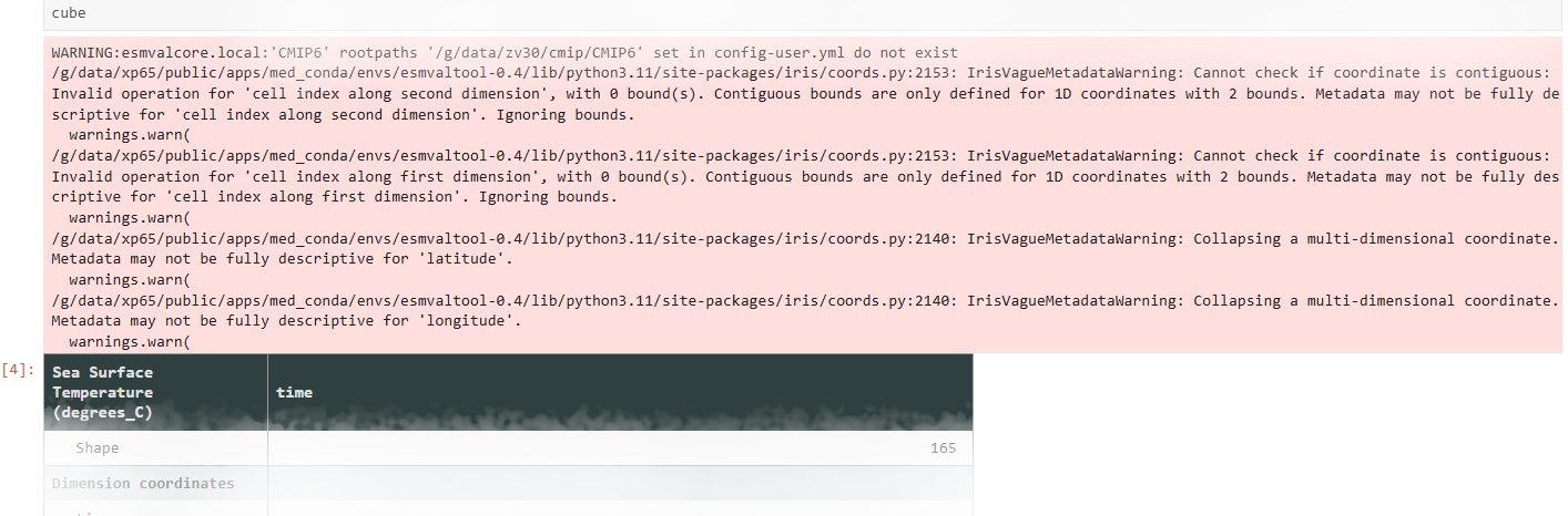
Note: Warnings
When the notebook cell runs you may get some warnings. These would be similar to what is in the main_log.txt and main_log_debug.txt files in the output of a recipe run. The warnings can come from any of the python libraries used to process the data. If they are just warnings the cell can still complete and return an output
Example warnings
Custom code
We have so far solely used ESMValCore, however, you can use your own custom code and
being in a Notebook means you can try straight away. Now, continue with other libraries
and make custom plots such as xarray.
import xarray as xr
da = xr.DataArray.from_iris(cube)
da.plot()
print(da)
Plot data
The output from the preprocessor functions are Iris cubes. Iris has wrappers for matplotlib to plot the processed cubes. This is useful in a notebook to help develop your recipe with the esmvalcore preprocessors.
from iris import quickplot
quickplot.plot(cube)
Build workflow and diagnostic
Exercise - Easy IPCC plot for sea surface temperature
Let’s pull some of these bits together to build a diagnostic.
- Using the
Datasetobject, make a template which we can use to find multiple datasets we want to analyse together for variabletos.- The datasets being
"CESM2", "MPI-ESM1-2-LR", "ACCESS-ESM1-5"and experiments'ssp126', 'ssp585'with historical, iterate to build a list of datasets.- Apply the preprocessors to each dataset and plot the result
Solution
import cf_units
import matplotlib.pyplot as plt
from iris import quickplot

from esmvalcore.config import CFG
from esmvalcore.dataset import Dataset
from esmvalcore.preprocessor import annual_statistics, anomalies, area_statistics


# Declare common dataset facets
template = Dataset(
   short_name='tos',
   mip='Omon',
   project='CMIP6',
   exp= '*', # We'll fill this below
   dataset='*',  # We'll fill this below
   ensemble='r4i1p1f1',
   grid='gn',
)

# Substitute data sources and experiments
datasets = []
for dataset_id in ["CESM2", "MPI-ESM1-2-LR", "ACCESS-ESM1-5"]:
   for experiment_id in ['ssp126', 'ssp585']:
       dataset = template.copy(dataset=dataset_id, exp=['historical', experiment_id])
       dataset.add_supplementary(short_name='areacello', mip='Ofx', exp='historical')
       dataset.augment_facets()
       datasets.append(dataset)

# Set the reference period for anomalies
reference_period = {
   "start_year": 1950, "start_month": 1, "start_day": 1,
   "end_year": 1979, "end_month": 12, "end_day": 31,
}

# Load, pre-process, and plot the cubes
for dataset in datasets:
   cube = dataset.load()
   cube = area_statistics(cube, operator='mean')
   cube = anomalies(cube, reference=reference_period, period='month')  # notice 'month'
   cube = annual_statistics(cube, operator='mean')
   cube.convert_units('degrees_C')

   # Make sure all datasets use the same calendar for plotting
   tcoord = cube.coord('time')
   tcoord.units = cf_units.Unit(tcoord.units.origin, calendar='gregorian')

   # Plot
   quickplot.plot(cube, label=f"{dataset['dataset']} - {dataset['exp']}")

# Show the plot
plt.legend()
plt.show()
Pro tip: Convert to recipe
We can use the helper to start making the recipe. A recipe can be used for reproducibility of an analysis. This list the datasets in a recipe format and we would then have to create the preprocessors and diagnostic script.
from esmvalcore.dataset import datasets_to_recipe
import yaml

for dataset in datasets:
    dataset.facets['diagnostic'] = 'easy_ipcc'
print(yaml.safe_dump(datasets_to_recipe(datasets)))
Output
datasets:
- dataset: ACCESS-ESM1-5
  exp:
  - historical
  - ssp126
- dataset: ACCESS-ESM1-5
  exp:
  - historical
  - ssp585
- dataset: CESM2
  exp:
  - historical
  - ssp126
- dataset: CESM2
  exp:
  - historical
  - ssp585
- dataset: MPI-ESM1-2-LR
  exp:
  - historical
  - ssp126
- dataset: MPI-ESM1-2-LR
  exp:
  - historical
  - ssp585
diagnostics:
  easy_ipcc:
    variables:
      tos:
        ensemble: r4i1p1f1
        grid: gn
        mip: Omon
        project: CMIP6
        supplementary_variables:
        - exp: historical
          mip: Ofx
          short_name: areacello
        timerange: 1850/2100
Run through Minimal example notebook
You can download an example notebook file here. This notebook includes:
- Plot 2D field on a map
- Hovmoller Diagram
- Wind speed over Australia
- Air Potential Temperature (3D data) Transect
- Australian mean temperature timeseries
Exercise: Sea-ice area
Use observation data and 2 model datasets to show trends in sea-ice.
- Using variable
siconcwhich is a fraction percent(0-100)- Using datasets:
dataset:'ACCESS-ESM1-5', exp:'historical', ensemble:'r1i1p1f1', timerange:'1960/2010'dataset :'BCC-CSM2-MR', exp:'piControl', ensemble='r1i1p1f1', timerange:'1960/2010'- Using observations:
dataset:'NSIDC-G02202-sh', tier:'3', version:'4', timerange:'1979/2018'- or use other
siconcobservations
- Extract Southern hemisphere
- Use only valid values (15 -100 %)
- Sum sea ice area which will be the fraction multiplied by cell area and summed
- Plot yearly minimum and maximum value
Solution notebook can be downloaded here.
1. Define datasets:
from esmvalcore.dataset import Dataset
obs = Dataset(
   short_name='siconc', mip='SImon', project='OBS6', type='reanaly',
   dataset='NSIDC-G02202-sh', tier='3', version='4', timerange='1979/2018',
)
# Add areacello as supplementary dataset
obs.add_supplementary(short_name='areacello', mip='Ofx')

model = Dataset(
   short_name='siconc', mip='SImon', project='CMIP6', activity='CMIP',
   dataset='ACCESS-ESM1-5', ensemble='r1i1p1f1', grid='gn', exp='historical',
   timerange='1960/2010', institute = '*',
)

pi_facets={'dataset' :'BCC-CSM2-MR', 'exp':'piControl', 'activity':'CMIP'}

model.add_supplementary(short_name='areacello', mip='Ofx')

model_pi = model.copy(**pi_facets)
Tip: Check dataset files can be found
The observational dataset used is a Tier 3, so with some licensing restrictions. Check files can be found for all the datasets:
for ds in [model, model_pi, obs]:
   print(ds['dataset'],' : ' ,ds.files)
   print(ds.supplementaries[0].files)
You can try to find and add another observational dataset. eg:
obs_other = Dataset(
   short_name='siconc', mip='*', project='OBS', type='*',
   dataset='*', tier='*', timerange='1979/2018')

obs_other.files
2. Use esmvalcore API preprocessors on the datasets and plot results
import iris
import matplotlib.pyplot as plt
from iris import quickplot
from esmvalcore.preprocessor import (
           mask_outside_range,
           extract_region,
           area_statistics,
           annual_statistics
)
# model_om - at index 1 to offset years

load_data = [model, model_pi, obs]

# function to use for both min and max ['max','min']

def trends_seaicearea(min_max):
   plt.clf()
   for i,data in enumerate(load_data):
       cube = data.load()
       cube = mask_outside_range(cube, 15, 100)
       cube = extract_region(cube,0,360,-90,0)
       cube = area_statistics(cube, 'sum')
       cube = annual_statistics(cube, min_max)
       iris.util.promote_aux_coord_to_dim_coord(cube, 'year')
       cube.convert_units('km2')
       label_name = data['dataset']
       print(label_name, cube.shape)
       quickplot.plot(cube, label=label_name)

   plt.title(f'Trends in Sea-Ice {min_max.title()}ima')
   plt.ylabel('Sea-Ice Area (km2)')
   plt.legend()

trends_seaicearea('min')
Key Points
API can be used as a helper to develop recipes
Preprocessors can be used in a Jupyter Notebook to check the output
Use
datasets_to_recipehelper to start making recipes